Appendix: Upwind scheme#
강좌: 기초 전산유체역학
Modified Wavenumber Analysis for Upwind scheme#
PDE Solution을 \(u(x, t) = \psi(t) e^{ikx}\) 로 생각한다.
이를 아래 Upwind 차분식에 적용하면 다음과 같다.
\[
\frac{du(x_j, t)}{dt} = - a \frac{u(x_j,t) - u(x_{j-1}, t)}{\Delta x}
\]
\[
\frac{d \psi}{d t} e^{ikx_j} = - \frac{a}{\Delta x} \left (e^{ikx_j} - e^{ik(x_j - \Delta x)} \right) \psi
\]
이를 정리하면
\[
\frac{d \psi}{d t} = - \frac{a}{\Delta x} \left (1 - e^{-ik\Delta x} \right) \psi
= -a i \frac{-i + i e^{-ik\Delta x}}{\Delta x} \psi = -a i k' \psi.
\]
차분식에 의해 Modified wavenumber \(k'\) 은 다음과 같다.
\[
k' = \frac{-i + i e^{-ik\Delta x}}{\Delta x}
\]
Stability 분석을 위해 모델 방정식 형태로 표현하면 \(\lambda=-iak'\) 를 분석하면 다음과 같다.
\[
\lambda = - i a k' = - \frac{a}{\Delta x} \left (1 - e^{-ik\Delta x} \right)
\]
Central 기법과 달리 복소수이다.
Stability Region#
앞서 구한 몇가지 ODE 에서 Stability region은 다음과 같다.
Euler Explicit#
\[
\sigma = 1 + z
\]
4차 정확도 Runge Kutta Method#
\[
\sigma = 1 + z + \frac{1}{2} z^2 + \frac{1}{6} z^3 + \frac{1}{24} z^4
\]
여기서 \(z=\lambda \Delta t\) 이다.
앞서 구한 \(\lambda\) 를 이용해서 분석하면 다음과 같다.
\[
z = \lambda \Delta t = -\frac{a \Delta t}{\Delta x} \left (1 - e^{-ik\Delta x} \right)
= -\nu \left (1 - e^{-ik\Delta x} \right)
\]
이 경우 대부분 실수 측에서 Stability 한계가 결정된다.
이를 확인하기 위해 수치적으로 \((\nu, k \Delta x)\) 에 대해 극좌표게로 분석 가시화 해본다.
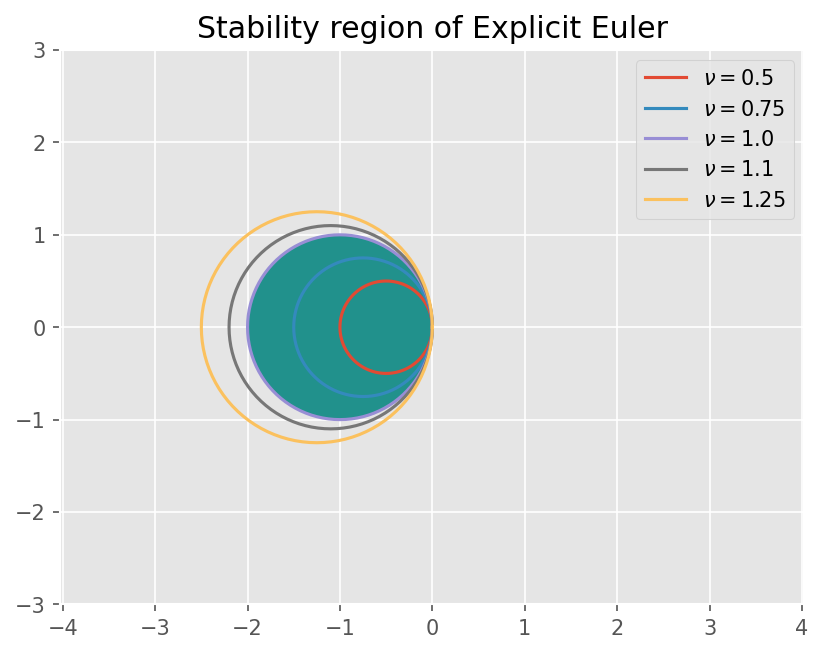
Euler Explicit#
Von nuemann 안정성 분석과 동일한 결과이다.
실수측 \(k \Delta x = 0, 180\) 일 때 \(\sigma\) 가 최대이다.
\(Real(z)\) 대해서만 분석하면
\[
Real(z) = -\nu (1 - \cos(k \Delta x))
\]
즉
\[
\min(Real(z)) = - 2 \nu
\]
Euler Explict의 최대 실수측 범위인 -2를 고려하면
\[
\nu \leq 1.
\]
%matplotlib inline
from matplotlib import pyplot as plt

import numpy as np

plt.style.use('ggplot')
plt.rcParams['figure.dpi'] = 150
# Make grid
x = np.linspace(-3, 3, 201)
y = np.linspace(-3, 3, 201)
X, Y = np.meshgrid(x, y)
z = X + Y*1j

# Amplication factor of Explicit Euler (z=lambda h)
sig = 1 + z

# Same scale of x and y
plt.axis('equal')

# Stability region
plt.contourf(X,Y,abs(sig), levels=[0, 1])

# Title
plt.title('Stability region of Explicit Euler')

# For CFL number
nus = [0.5, 0.75, 1.0, 1.1, 1.25]
for nu in nus:
    theta = np.linspace(0, 2*np.pi, 101)

    # Amplication factor
    z = -nu *(1 - np.exp(-theta*1j))

    plt.plot(z.real, z.imag)

plt.legend([r'$\nu={}$'.format(nu) for nu in nus])
<matplotlib.legend.Legend at 0xfb5ba1d4fb60>
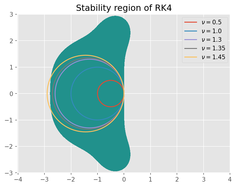
4차 정확도 Runge Kutta Method#
Von nuemann 안정성 분석과 동일한 결과이다.
실수측 \(k \Delta x = 0, 180\) 일 때 \(\sigma\) 가 최대이다.
\(Real(z)\) 대해서만 분석하면
\[
\min(Real(z)) = - 2 \nu
\]
Euler Explict의 최대 실수측 범위인 -2.79를 고려하면
\[
\nu \leq 1.395.
\]
# Make grid
xx = np.linspace(-3, 3, 201)
yy = np.linspace(-3, 3, 201)
X, Y = np.meshgrid(xx, yy)
z = X + Y*1j

# Amplication factor of RK4 (z=lambda h)
sig = 1 + z + 0.5*z**2 + z**3/6 + z**4/24

# Same scale of x and y
plt.axis('equal')

# Stability region
plt.contourf(X,Y,abs(sig), levels=[0, 1])

# Title
plt.title('Stability region of RK4')

# For CFL number
nus = [0.5, 1.0, 1.3, 1.35, 1.45]
for nu in nus:
    theta = np.linspace(0, 2*np.pi, 101)

    # Amplication factor
    z = -nu *(1 - np.exp(-theta*1j))

    plt.plot(z.real, z.imag)

plt.legend([r'$\nu={}$'.format(nu) for nu in nus])
<matplotlib.legend.Legend at 0xfb5b9f413d90>